🚀 Quickstart#

In this quickstart guide, we describe how to use deshift to solve distributionally robust optimization (DRO) problems of the form

\[ \min_{w \in \mathbb{R}^d} \max_{q \in \mathcal{Q}} q^\top \ell(w) - \nu D(q \Vert \mathbf{1}/n) \]

where:

$w$ denotes the parameters of a model (the “primal variables”),
$q$ denotes the weights on individual training examples (the “dual varialbes”),
$\ell: \mathbb{R}^d \rightarrow \mathbb{R}^n$ denotes a loss function for individual training examples,
$D(\cdot \Vert \mathbf{1}/n)$ denotes a divergence (either Kullback-Leibler or $\chi^2$) between a distribution on $n$ atoms and the uniform distribution $\mathbf{1}/n = (1/n, \ldots, 1/n)$,
$\nu \geq 0$ is a dual regularization parameter, or the “shift cost”,

The package requires only a single line of additional code; we first import a constructor function that specifies our choice of ambiguity set, which is chosen to be spectral risk measures in this case.

import numpy as np
import matplotlib.pyplot as plt
import seaborn as sns

import sys
sys.path.append("../..")
from deshift import make_spectral_risk_measure, make_superquantile_spectrum

The fundamental object required to compute the gradient of the DRO objective is a function that computes

\[ l \mapsto \operatorname{argmax}_{q \in \mathcal{Q}} q^\top l - \nu D(q \Vert \mathbf{1}_n/n) \]

for some vector $l \in \mathbb{R}^n$. In particular, we set

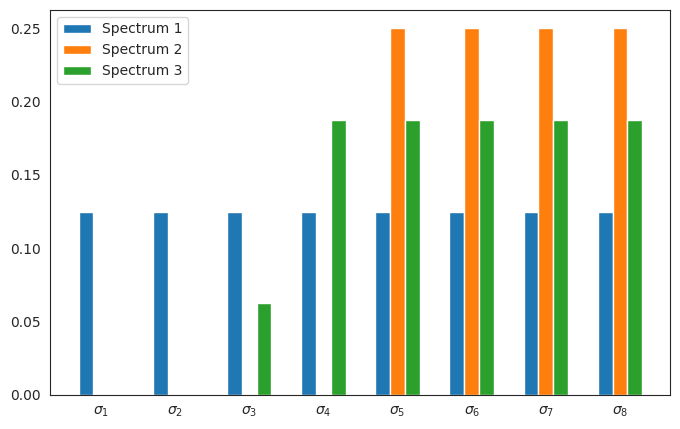
\[ \mathcal{Q} \equiv \mathcal{Q}(\sigma) = \operatorname{conv}\{\text{permutations of $\sigma$}\}, \]

where $\sigma = (\sigma_1, \ldots, \sigma_n)$ is a vector of non-negative weights that sums to one, called the spectrum. We call $\mathcal{Q}(\sigma)$ is the permutahedron associated to the vector $\sigma$. Various choices of $\sigma$ can be generated by using the make_<spectrum_name>_spectrum functions within the package, which return Numpy arrays with value equal to $\sigma$. Each has a risk parameter which determines the skewedness of the spectrum (which influences the size of $\mathcal{Q}(\sigma)$).

batch_size = 8

sns.set_style("white")
fig, ax = plt.subplots(1, 1, figsize=(8, 5))

offset = 0.2
colors = ["tab:blue", "tab:orange", "tab:green"]
x = np.arange(batch_size)
for i in range(3):
    spectrum = make_superquantile_spectrum(batch_size, 1.0 / (i + 1.))
    ax.bar(x + i * offset, spectrum, color=colors[i], width=offset, label=f"Spectrum {i + 1}")
ax.legend(loc="upper left")
ax.set_xticks(x + offset)
ax.set_xticklabels([r"$\sigma_1$", r"$\sigma_2$", r"$\sigma_3$", r"$\sigma_4$", r"$\sigma_5$", r"$\sigma_6$", r"$\sigma_7$", r"$\sigma_8$"])
plt.show()

_images/a5645478b2fa6d308c0cc359bc18bb8f72c6a37283f27f505c174aa41c8131aa.png

To create the oracle that performs the maximization, we simply use the make_spectral_risk_measure function and specify the form of the penalty with the penalty parameter and the shift cost $\nu \geq 0$ with the shift_cost parameter. Currently, the $\chi^2$-divergence penalty is supported by using the chi2 string and the Kullback-Leibler using the kl string.

batch_size = 10
shift_cost = 1.0
penalty = "chi2" # options: 'chi2'

# define spectrum based on the 2-extremile
spectrum = make_superquantile_spectrum(batch_size, 0.5)

# create function which computes weight on each example
compute_sample_weight = make_spectral_risk_measure(spectrum, penalty=penalty, shift_cost=shift_cost)

The result will be a function that takes in a collection of losses and returns a weight associated with each loss. As a sanity check, the sorted order of the weights should be the same as the sorted order of the losses.

np.random.seed(123)

losses = np.random.normal(size=(batch_size,))
weights = compute_sample_weight(losses)

print(weights[np.argsort(losses)])

---------------------------------------------------------------------------
AssertionError                            Traceback (most recent call last)
Cell In[4], line 4
      1 np.random.seed(123)
      3 losses = np.random.normal(size=(batch_size,))
----> 4 weights = compute_sample_weight(losses)
      6 print(weights[np.argsort(losses)])

File /opt/hostedtoolcache/Python/3.11.13/x64/lib/python3.11/site-packages/deshift/_src/spectral_risk.py:29, in make_spectral_risk_measure.<locals>.max_oracle(losses)
     28 def max_oracle(losses):
---> 29     assert torch.is_tensor(losses), "`losses` must be a PyTorch tensor"
     30     with torch.no_grad():
     31         device = losses.get_device()

AssertionError: `losses` must be a PyTorch tensor

As seen above, the result is a PyTorch tensor. This is made to be amenable to existing PyTorch training workflows. See the train_fashion_mnist.ipynb example for guidance on embedding these weights into an existing PyTorch training loop with backpropagation.